Contents
- Index
- Previous
- Next
Smoothing Windows
If a sinewave is passing through zero at the beginning and end of the time series, the resulting FFT spectrum will consist of a single line with the correct amplitude and at the correct frequency. If, on the other hand, the signal level is not at zero at one or both ends of the time series record, truncation of the waveform will occur, resulting in a discontinuity in the sampled signal. This discontinuity causes problems with the FFT process, and the result is a smearing of the spectrum from a single line into adjacent lines. This is called "leakage"; energy in the signal "leaks" from its proper location into the adjacent lines.
Leakage could be avoided if the time series zero crossings were synchronized with the sampling times, but this is impossible to achieve in practice. The shape of the "leaky" spectrum depends on the amount of signal truncation, and is generally unpredictable for real signals.
In order to reduce the effect of leakage, it is necessary that the signal level is forced zero at the beginning and end of the time series. This is done by multiplying the data samples by a "smoothing window" function, which can have several different shapes. The difference between each smoothing window is the way in which they transition from the low weights near the edges to the higher weights near the middle of the sequence. If there is no windowing function used, this is called "Rectangular", "Flat", or "Uniform" windowing.
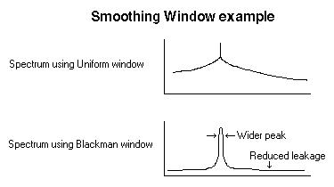
While the smoothing window does a good job of forcing the ends to zero, it also adds distortion to the time series which results in sidebands in the spectrum. These sidebands, or side lobes, effectively reduce the frequency resolution of the analyzer; it is as if the spectral lines are wider. The measured amplitude of the weighted signal is also incorrect because a portion of the signal level is removed by the weighting process. To make up for this reduction in power, windowing algorithms give extra weight to the values near the middle of the sequence.
The figure shown below compares the spectrum of a signal using a Uniform window and a Blackman window. Remember that a Uniform window is actually no window at all.
Characteristics of various smoothing windows
Window Frequency Amplitude Leakage
Type Resolution Resolution Suppression Application
Bartlett Fair Fair Moderate
Blackman Fair Good Excellent Distortion Measurements
Exponential Fair Fair Poor Transient measurements such as impact hammer tests (use for the accelerometer input channel)
Flattop Poor Excellent Moderate Accurate Amplitude measurements
Force Fair Good Poor Impact Hammer tests (use for the impact hammer input channel)
Hamming Fair Fair Fair
Hanning Fair Excellent Excellent Distortion measurements, Noise measurements
Kaiser Fair Fair Poor
Parzen Fair Fair Poor
Triangular Fair Fair Poor
Uniform Excellent Poor Poor High resolution frequency measurements, Impulse response measurements
Gaussian Excellent* Fair Fair Allows very high frequency resolution using gaussian interpolation*
*Gaussian interpolation is used for the Peak Frequency Utility, Data Logging and Automation Peak Frequency values.
Advanced Window Settings
Clicking the "Advanced Settings" button allows you to specify additional parameters for certain window types. For more information please refer to the following links:
https://en.wikipedia.org/wiki/Window_function
https://en.wikipedia.org/wiki/Kaiser_window
https://en.wikipedia.org/wiki/Exponential_decay
Notes:
The Time Series View displays the signal prior to the application of any smoothing window except when previewing trigging waveform.
The effects of these functions are most noticeable when using Logarithmic scaling.
When Independent Scaling and Calibration is enabled you can select different smoothing windows for each channel
See also: Scaling, FFT size, Overlap Processing , Sampling Rate